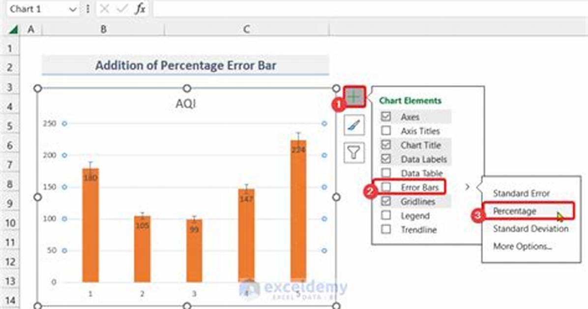
Apart from Windows, you can also add Excel error bars for Mac, but with a different yet straightforward path and process:
- Click on your data or chart, then proceed to Chart Design tab on the header.
- Go to the Add Chart Element, select to bring options in the drop-down.
- Continue navigating through the same path as in Windows and press OK after completing the procedure.
- The changes will be effected immediately on the data.
If you want to customize your values, the same process applies as in Windows:
- Instead of choosing your preferred type as above, explore more options on the bottom of the drop-down.
- Proceed to the new window and move down to the Error Amount section in the new window, click Custom and then the Specify Value option.
- Fill the two parts in the small window with your positive and negative values.
- Type your preferred figures and then click OK to make changes in the chart.
You are now familiar with how to add error bars in Excel both for Windows and Mac operating systems. You can now easily add the tool in your chart or graphical presentation. Reach out to friends and colleagues and help them when they stranded on what to do. Maybe one day the skill may earn you some cash somewhere.
READ ALSO: How to find and remove duplicates Excel: Tutorial
Source: Legit.ng